07/30/2025
Controlling cooling water flow is a critical element of high-performance cooling systems. Fortunately, pressure is a straightforward measurement that can be used as a cost-effective control input for flow control systems. Proper interpretation of pressure readings is required for accurate control at desired rates. This article covers pressure reading methods, control strategies and practical tips.
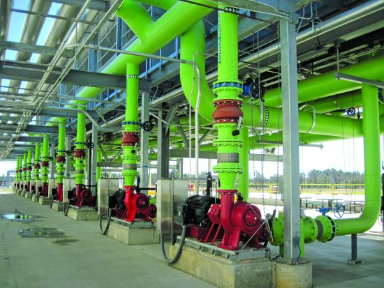
This cooling tower pump system uses single-pressure flow control in multiple application loops.
Process cooling systems are linked systems of devices that remove heat from machines and process materials. Because process requirements can be variable and equipment condition changes over time, the components of these linked systems are designed with various control functions to enable cooling operations to meet the required needs without over- or under-cooling, neither of which is desirable.
Under-cooling of equipment or product could result in machines overheating or incompletely cooled and consequently off-spec products. Over-cooling can result in excessively long cycle times and inefficient operation from required product reheating or excessive cooling equipment operation. Given the alternatives, many systems tend toward over-cooling with the use of additional devices to mitigate potential ill effects. While functionally adequate, this results in further total system complexity and even lower system efficiency.
The generally changeable aspects of heat transfer that underlie process cooling are (1) the temperature difference between the cooling medium and the cooled device or material and (2) the flow rate of the cooling medium. Note that many other factors are part of the complete cooling system function, such as the heat exchanger designs and materials and the selection of the cooling medium, but these are all assumed to be fixed and established in any given situation. Practically speaking, the only elements we have immediate control over are the temperatures and flows.
Cooling system temperatures are typically controlled by the settings on chillers or cooling towers, and this is commonly recognized and used in cooling system design to achieve desired operation and performance. For more on optimizing temperatures, read our previous article “Evaluating Process Cooling Supply Temperatures”.
Typical Flow Conditions in Cooling Systems
The other commonly controllable component, flow, is not often controlled directly. Instead, pumps are selected and systems designed to provide pressures expected to result in adequate flows. Because pressure is straightforward to measure, it is easy to determine pumps’ output pressure (“head,” more precisely, but convertible to and measured in cooling systems as pressure) and the pressure at different points in a system. These systems are started up and, as long as everything seems to work well enough, little additional thought is given to the operation.
It is extremely common to see pressure gauges on the suction and discharges of pumps, the in and out points of system machines, and at other points of interest in a cooling system. Pressure gauges are relatively inexpensive and frequently fitted with good range decals showing the acceptable ranges for given devices.
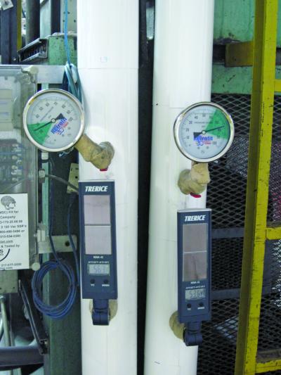
These gauges include decals showing the normal range of operation.
Unfortunately, the pressure, and, consequently, the flow, are somewhat random in many systems depending on how many pumps are on and how many lines are operating. Operators typically watch the pressure gauges and turn pumps on or off as needed to stay in a target range. This requires vigilance for consistency. It’s seldom maintained at night and on weekends.
This “fiddle factor” manual operation results in potentially significant variations in the actual flow to any given device, making the actual cooling effect inconsistent over time. Integrated Services Group (ISG) has observed pressure variations of as much as 2:1 in many systems when evaluating plants, and +/- 30-50% variations are common in uncontrolled operations.
Potential for Constructive Pressure Control
Because pressure and flow are linked, pressure can be used intelligently to control flow. This requires understanding the relationship between pressure and flow, then using that understanding to implement pressure control functions to enable reasonably accurate flow management. Using pressure control well allows plants to control flows to individual devices to a narrow range of potentially +/- 5-10%, depending on the distribution piping design, plant size and other factors. The resulting stable operation is what really matters in production operations.
Note that system design can play a critical role in the ability of plants to have uniform pressure and flow throughout their systems, however, that subject is beyond the scope of this article. Many historical approaches to piping system design were based on material economy and not process uniformity and energy efficiency. In many cases, there are significant opportunities to improve the piping in new systems or system modifications.
When considering the use of pressure as a proxy for flow, several questions arise:
- What is the correct flow and how do plants verify thIs?
- Is this a constant value or does it change?
- How much pressure is needed for the correct flow?
- How do plants control pumps to nsure the required pressure?
This article will address these questions.
The Relationship Between Pressure and Flow
Perhaps surprisingly, pressure and flow are not linearly related. In other words, doubling pressure does not double flow. Instead, there is a flow-squared to pressure relationship. This means, for a given device (a heat exchanger, valve or other fitting and even a straight run of pipe), doubling flow requires increasing pressure by four times!
Looking strictly at the motivating pressure and flow, and assuming a constant system (no control valve operations or other dynamic changes to the flow system), the following equation applies
P2=P1×ã(F2/F1)ã^2
Or, to solve for the flow resulting from a pressure change
F2=F1×√(P2/P1)
This means doubling the portion of the pressure being used to actually drive (or motivate) the flow, not the total measured pressure which may include other factors such as closed system minimum pressures (from the expansion tank and make-up water control) and fixed elevation components in systems with elevated cooling towers or tanks.
This concept can be graphically displayed as follows for prototypical flow systems:
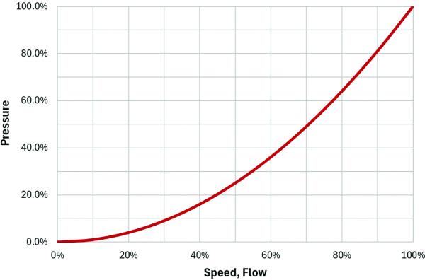
The curve for an ideal flow pressure.
In a simple closed system with fixed components (including pumps, piping and heat transfer devices) where the pump is speed-controlled with a variable frequency drive (VFD), the flow varies linearly with the pump speed within a normal flow range while pressure varies as described previously. The required pump power varies according to the power to flow cubed relationship described in detail in the “Pump and Fan Affinity Laws Power Calculations” sidebar in the article “Holistic Controls for Superior Cooling Systems Efficiency, Pt.2” (May 2024).
Pressure Measurements in Cooling Systems
It is vital when using pressure measurements as control inputs to correctly understand what the reading means and what part of it is the flow-motivating component.
Consider the example of a pump discharge pressure gauge showing 60 psi (4.1 barg). If this pump is connected to a ground-level tank that is open to the atmosphere and to which the process flow returns, then approximately the entire 60 psi (4.1 barg) is available to drive the system flow. (For clarity, this article ignores modest elevation differences, such as the fluid level in the tank or the height of the pressure sensor. In practice, these should be considered to maintain the best possible accuracy.)
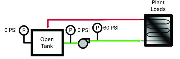
The schematic for a simple flow loop.
If the pump is connected to a suction header in a closed system with a reference pressure setting of 30 psi (2.1 barg) – the make-up water pressure control valve and expansion tank are set to 30 psi (2.1 barg) – and it has the same 60 psi discharge pressure, then the system only has 30 psi (2.1 barg) to create the flow. The pump doesn’t have to work as hard to reach the 60 psi (4.1 barg) so the power will be lower, but the focus here is on the pressure indication. That’s what we have to understand for pressure-flow control operation.
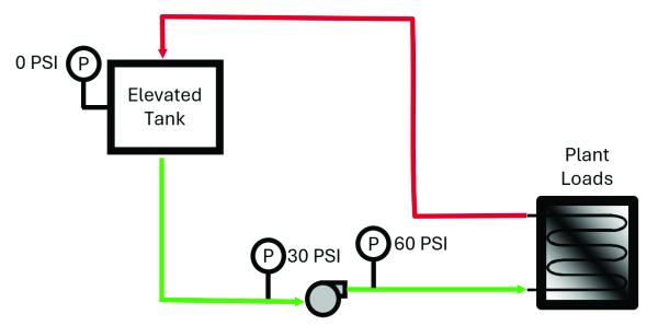
Flow loop example schematic with above-zero reference pressure.
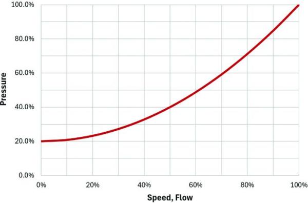
Flow and pressure graph illustrating above-zero reference pressure.
Even though the two gauges read the same discharge pressure, the two systems’ flow capability is significantly different. The good news is the difference isn’t half, as the pressure-to-flow relationship is not linear. Using the formula from above and the two net flow motivating pressures from the examples, the flow in the closed system would be approximately 71% of the open system flow.
F2=100%×√(30/60)=70.7% of F1
Whether this is enough flow depends on the specific circumstances. In any case, this clearly illustrates that the key challenge in analyzing and controlling pressure, and hence flow, is understanding and measuring the correct pressure values.
Differential Pressure Measurements
As noted previously, the effective pressure driving the flow, and which must be controlled, is most often not the same as the readily readable gauge pressure in typical locations, such as at the pump outlet or discharge header, or at the inlet to cooled devices such as refrigeration compressors, chillers or process machinery. The simple gauge pressure must be adjusted to account for various elements of the total system, such as:
- Elevation of the water (the weight of the water and the height of the system)
- External pressure inputs such as make-up water and/or expansion tanks
- Required pressure to return the water to the cooling equipment
The confusion about how much pressure is usefully available arises in different situations, such as when a system is pumping to an elevated location such as a cooling tower above a roof, or in a closed, pressurized system. For this reason, in many cases the ideal pressure measurement for control is one between the supply piping and the return piping in a relevant location.
Differential pressure (DP) measurement uses a pressure transducer reading the difference in pressure between two separate points, commonly between a supply pipe and a return pipe, although these sensors are also frequently used to read pressure drop across particular devices such as chillers and heat exchangers. (In a sense, all pressure readings are differential readings, as conventional single pressure gauges and transducers read the difference between the measured pressure and the local atmospheric pressure.)
DP is calculated simply as
DP=P high-P low
and shares the same psi units as single-pressure readings.
For distribution system DP, the two pressure connections will be on the supply and return pipes, giving the difference between the two pipes and indicating the actual pressure available to induce flow in the connected equipment. Reading the DP across a particular device requires connecting the DP sensor to the cooling water inlet and outlet piping. This negates the effect of external system pressures. The remaining DP reflects the actual pressure difference through the device.
![]()
A differential pressure transducer with a three-valve manifold and piped blowdowns.
Using DP readings across devices is an affordable and cost-effective means of showing flow through critical items including chillers and heat exchangers. However, the DP reading must be initially calibrated using a reliable means – such as a clamp-on flow meter – and periodically checked to maintain accurate flow readings. This is described further below.
Pressure Measurements Selection for Control in Cooling Systems
In control system design, part of the challenge is selecting the ideal pressure measurement for each control application. The choice of pressure measurement type (single vs. DP) includes several factors that must be balanced in each case. These include:
- Appropriate reading: Does the basic reading type correctly indicate (possibly with some mathematical modification) the needed condition? This can vary depending on how the controls will use the input.
- Location: Does the connection location properly measure the reading desired?
- Quantity: Will a single reading be adequate or are multiple readings necessary for the required control? Some applications are best performed using several sensors and “low man” control, such as with different departments in a multi-process plant or large systems with different standard conditions.
- Accessibility: Can the sensor be installed and connecting piping run to enable routine maintenance of the sensor and the piping?
- Cost: Does the selected type of sensor, the particular device and the installation approach meet the requirements at a reasonable cost?
In general, DP sensing is the most certain method for obtaining satisfactory results. In some cases, there are less expensive and simpler approaches that can be applied to sensors while meeting requirements. For example, a single chiller condenser cooling application with an elevated cooling tower could be reasonably controlled using a typical single pressure sensor at the chiller inlet if (1) the piping in the system is sufficiently large so flow losses are modest compared to the elevation head, and (2) the tower return is to open top basins with essentially no backpressure variation with flow (spray nozzles would not meet this criterion). In this case, the controls can subtract the elevation head from the read value and derive a useful indication of the actual condenser pressure drop.
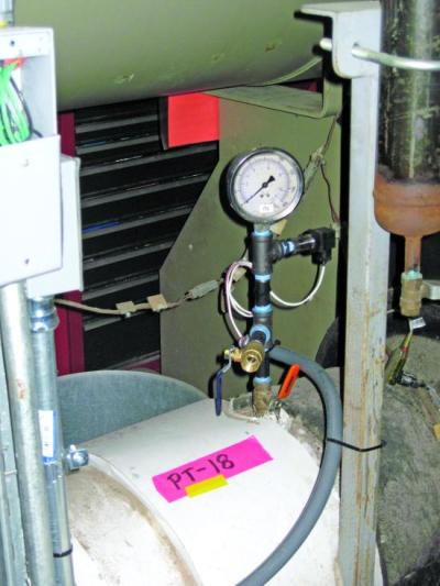
This single pressure sensor installation includes a manual blowdown port and gauge.
Part of the decision process is considering the impact of the reading. An approach that would be fully justified on a system controlling several 200 horsepower (hp) pumps for a whole plant system might not make sense if it were only on a single 25 hp pump simple loop system.
Using Pressure Measurements for Control
While the pressure reading quality is vital, the control application logic is equally important for effective pressure-based control. The two elements must function correctly together to achieve satisfactory flow control of the actual cooling loads in the plant. Critically, control program performance must remain stable throughout the operating range of the particular applications.
This can be challenging given the underlying flow change-squared relationship between pressure and flow. This non-linearity can cause control stability issues in applications with large operating ranges, which cooling system controls often encounter given the typically expected variations in operation. These include machines turned on and off (from five-day/two-day schedules, seasonal output variations and evening schedules), seasonal temperatures resulting in opportunities for variable flow (resulting in pump savings) and other inherent aspects of cooling systems operation.
These load (and consequently flow) variations can result in common speed control ranges of 70-95% in many systems. ISG has often implemented speed ranges of 40-100% in efficient closed loops with high efficiency design. Appropriate control logic function selection is critical in these instances to have stable, correct speed control performance.
When done poorly, pressure-based speed control results in hunting, where the speed output continuously cycles between high and low values, and jumpy systems where the speed output is inconsistent and unstable. Either of these conditions leads to the controlled pumps’ VFDs being put in hand, and the entire benefit of the effort is lost.
One additional, frequently critical, step in commissioning pressure control logic is calibrating the required pressure to the target flow, for example when setting up chiller condenser pumps and other specific device configurations. This is typically done using temporary flow meters to set control pressure setpoints or ranges correlated to the desired flows. This step is not used on every device in a system-wide control application as there are too many potential control points for device-specific calibration. Instead, readings at representative sample devices are used to develop the required pressure at the specific sensing locations for the required overall system flows.
Several control logic approaches can be applied in various cases, irrespective of the type of pressure sensing. Examples include:
Single setpoint PID control: Using the pressure reading in a PID function to adjust pump speed. This is the most common use found, but it can be unstable in some cases. Up and down hunting often results in widely variable applications.
Multiple single-setpoint PID control: Using two or more instances (typically not more than 4 or 5) of pressure readings through independent PID functions and control off the higher calculated speed (the point with the greatest negative deviation from setpoint). This can also lead to hunting, but with potentially multiple, overlapping instances.
Linear range control: Using the pressure input to a linear output range, where the pressure directly correlates to an output speed. This simple approach is typically applied in small systems with a narrow pressure input range over an inverse speed output range. For example, 50 psi (3.4 barg) equals 51 Hz while 48 psi (3.3 barg) equals 60 Hz. The two psi input variation results in a 15% pump speed change with the lower pressure driving the higher pump speed. This method gives a near flat flow output over a fairly wide flow range in fixed flow loop applications such as with multiple chiller condensers or refrigeration compressors. However, the devices must have similar flow-pressure drop characteristics.
Hybrid or enhanced methods: Using the pressure with some modifications or adjustments (such as subtracting an expansion tank pressure reference) as an input to one of the preceding approaches. These methods can provide capable flow control but can also be complicated and erratic if not carefully implemented.
The choice of different logic approaches is influenced by the general application and other potential complexities, such as an elevation offset. In addition to being fundamentally sound, the control logic in each case must also yield good results, with the system stable and performing as desired. Different approaches can be taken to improve the performance of control functions such as:
PID dampening: Adjust the PID settings, such as the cycle time or proportional, integral, derivative factors to slow down an erratic system. This must be used cautiously, as it can result in a system that is too slow to respond to significant input changes, such as major step load additions or incremental pumps starting.
Multi-step range PIDs: Using two or more – typically no more than three or four – separate and independent PID functions with linked step ranges where the input forces the selection of one PID’s output based on the input range. For example, three PIDs where one is selected for the input range of 20 (1.4 barg) or less to 30 psi (2.1 barg), one from 30-40 psi (2.1-2.8 barg), and one from 40 psi (2.8 barg) and above. Each PID can be tuned in a respective range for good performance to minimize the non-linearity of the pressure input’s effect on the resulting flow.
Algebraic input modification: Applying adjustments or other modifications to the pressure reading to improve the performance of the control logic. This would be in addition to other basic adjustments such as subtracting an elevation offset.
The challenge in many cases is having the control logic perform as required and still be comprehensible to the system operators and other users. Understanding how it should work is necessary so users can assess normal performance and adjust setpoints as needed. If the system can’t be understood, it will likely be overridden to a fixed speed, defeating the point of the controls. This happens more often than one would hope!
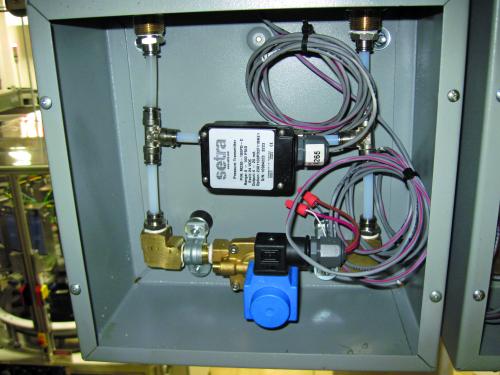
Practical Tips for Pressure Measurements in Cooling SystemsOnce the decision is made to use pressure inputs for control, there are a variety of steps that can be taken to improve the quality of the readings and the longevity of the sensors. In general, the following tips will help ensure and maintain good pressure control results for the long term. 1. Select high-quality devices within reason. There is no need for ¼% accuracy, heavy industry-type devices (which typically cost over $2000 for a single pressure sensor), as proper installation and maintenance are more important than extreme precision. Good quality HVAC devices of ½ to 1% accuracy (which typically cost under $500 for a single pressure sensor) are satisfactory. 2. Install with larger piping for a lower chance of blockage. Use a minimum of ½-inch diameter pipe for total connection loop lengths (supply pipe to sensor and back to return pipe) of 50 feet or less, and ¾-inch pipe over 50 feet. Do not use ¼ or 3/8-inch tube for the loop or there won’t be enough flow to periodically purge the loop to ensure good readings. 3. Pay particular attention to blowdown capabilities. Cooling tower loops that can pick up ambient dust and debris are highly susceptible to fouling on both single-pressure and DP applications, as particulates can collect in the pressure sensing connections and plug the pipes. This is extremely common in practice. Fully closed chilled water systems are less likely to have this problem, but they still need to be purged periodically. Purge open systems monthly or quarterly, and closed systems semi-annually or annually. 4. Regularly perform manual or automatic blowdown. Institute maintenance work orders to manually blow down the sensor loops (which requires bypass valving to allow flow through the piping while isolating the sensor) or implement an automatic blowdown for improved long-term reliability.
This ISG packaged DP sensor assembly includes automatic blowdown.
5. Don’t always use a DP sensor. Some applications can use a single pressure sensor with good results and lower installation costs. This requires clearly understanding the application and measurement components. 6. Do not use pump skid-located sensors. Unless in specific locations where the application supports their use on or near the pumps, avoid these sensors. Many factory-packaged solutions use integrated sensors with VFDs, and while these are better than across-the-line pump operation and no pressure sensing, they do not deliver the results available from more effective pressure sensing. |
Conclusion
Effective flow control is vital to satisfactory cooling system performance. Properly applied, pressure-based control is a cost-effective and reliable means of managing flows. This article has laid out the theoretical basis for using pressure-based control, described methods of measuring and applying pressure sensing inputs in control systems and provided field-proven practical tips for implementing and operating these controls.
About the Author

Clayton Penhallegon, Jr. is President and Managing Member of Integrated Services Group, which specializes in industrial cooling water system operational effectiveness and cost reduction. He has worked for over 35 years with various industries including plastics, paper, wood products, metal containers, and textiles. He holds a Bachelor of Mechanical Engineering from Georgia Tech, an MBA from Georgia State University and is a registered PE in Georgia.
About Integrated Services Group
Integrated Services Group performs industrial cooling water system operational effectiveness and cost reduction technical services. Its services include system assessments, new and upgrade system design, system start-up and retrocommissioning and high efficiency control design and implementation. ISG celebrated its 25th anniversary in 2022 and serves clients throughout North America. For information, visit https://www.isg-energy.com.
For similar articles on Cooling Controls System Assessments, please visit https://coolingbestpractices.com/system-assessments/cooling-controls.
Visit our Webinar Archives to listen to expert presentations on Cooling Controls System Assessments at https://coolingbestpractices.com/magazine/webinars.